CS 194-26: Image Manipulation and Computational Photography

Project Seven Part One - Homographies and Panoramas

Giulio Zhou

Background

Back when I was a kid, I used to go on all sorts of hiking trips. I have many fond memories of reaching the top of a trail and snapping all sorts of photos. One day, I saw my dad turning in a circle slowly, taking a bunch of photos. Puzzled, I asked him what he was doing and he told me that he was taking a panorama. After seeing the amazing results, I couldn't help but wonder how exactly this was possible. Many years later, I get a Nexus 6, take some pictures on a few outings and notice some very nice automatically generated panoramas, courtesy of Google Photos. This once again piqued my fascination, but in a different way. How exciting that we get to explore all of these techniques in this project! In this part, we explore the concept of homography, or projective transforms, which enables us to perform all the necessary mappings for image rectification and panorama generation. Let's start by taking a look at the transformation matrix.

Recall in the HW5 when we performed face morphing using linear transformations of triangles. This matrix looks awefully familiar, but with a couple of key differences. The bottom two zero terms now take on actual values! Not only does this enable scaling and rotation, but we can now warp the image as well. So, why go to all this trouble? Why don't we just find correspondence points and match them directly using some Sum of Squared Differences cost metric? Well, let's take a look at the results (recall from lecture).

Terrible, isn't it? The reason why this doesn't work is due to distortions from perspective. Instead, we'll do something a bit more clever. Using projective transforms, project all images onto the same projection plane (associated with that of the center image) and blend the boundaries. As I will show below, this produces far better results.

Part One: Image Rectification using Homographies

First, let's see how we can use homographies to perform image rectification of objects.

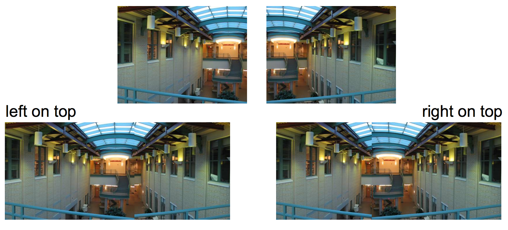
A view of the Palazzo lobby from my stay over the summer.	The floor pattern looked rather interesting, let's take a closer look.
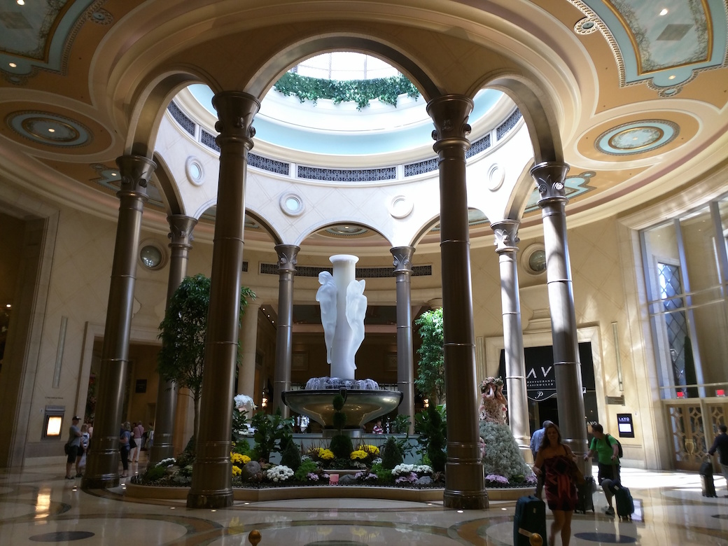
A front view of my Macbook.	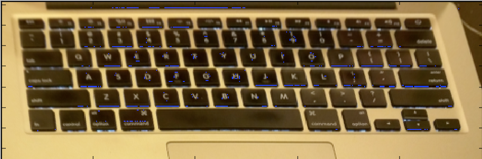Hey, I can see my keyboard from way up here!

Part Two: Image Stitching with Manual/Automatic Point Selection

Using the techniques from Part One, we can construct panoramas by projecting all of the source images onto the same projection plane, I begin by defining correspondence points between the two images (which may be done manually or automatically), aligning the resulting images, and then blending. Automatic correspondence point detection and matching occurs through the following steps.

Corner Detection: Using the Harris corner detector, find candidate corners then take just the top 100 corners using Adaptive Non-Maximal Suppression.
Extract Feature Descriptors: Extract a surrounding 40x40 pixel block around each descriptor, then blur and subsample to get an 8x8 feature descriptor.
Feature Matching: Between two images, compute all pairwise sum-of-squred-differences cost between their respective feature descriptors and keep all matches such that the first nearest neighbor has cost less than or equal to 0.7 times that of the second nearest neighbor.
Compute Homography: Run RANSAC for 1000 iterations and use the homography matrix that produces the greatest number of inliers.

Corner Detection Results

Once I obtained the corner points using the Harris corner detector, I used Adaptive Non-Maximal Suppression to obtain a more even distribution of feature points. This works by taking each point, computing the maximum radius for which it is a local maximum, sorting in descending order of radii then keeping the top N entries. As we can see, this helps us obtain a significantly better distribution of feature points.

Golden Gate Harris Corners	Golden Gate Harris Corners with suppression
Plane Harris Corners	Plane Harris Corners with suppression

Feature Matching Results

After acquiring the feature points and extracting the local pixels at each point, our next job is to automatically define correspondences between two images. This is done by comparing a feature descriptor's first and second nearest neighbors and using the "Russian Granny Algorithm", where we only consider a pair to its first nearest neighbor a match if it's cost is less than 0.7 times that of the second nearest neighbor.

Golden Gate Feature Matching

As seen above, there are a lot of mistakes in this image, likely due to the fact that this scene does not have many well-defined feature points and since many of the feature points look very similar. While choosing points manually produced a good result in Part One, it didn't look so good here. As such, I included an additional result.

Plane Left-to-Center Feature Matching	Plane Center-to-Right Feature Matching
Boston Left-to-Center Feature Matching	Boston Center-to-Right Feature Matching
MIT Left-to-Center Feature Matching	MIT Center-to-Right Feature Matching

Not too bad! Even though there were some apparent outliers in the end, we will see that the transformation matrix worked pretty well in the end, since there were a sufficient number of good points.

Manual/Automatic Panorama Results

Over the summer, I took a trip to San Francisco and got a few nice panoramas courtesy of Google photos. Here, I tried recreating them using transforms as we learned in class.

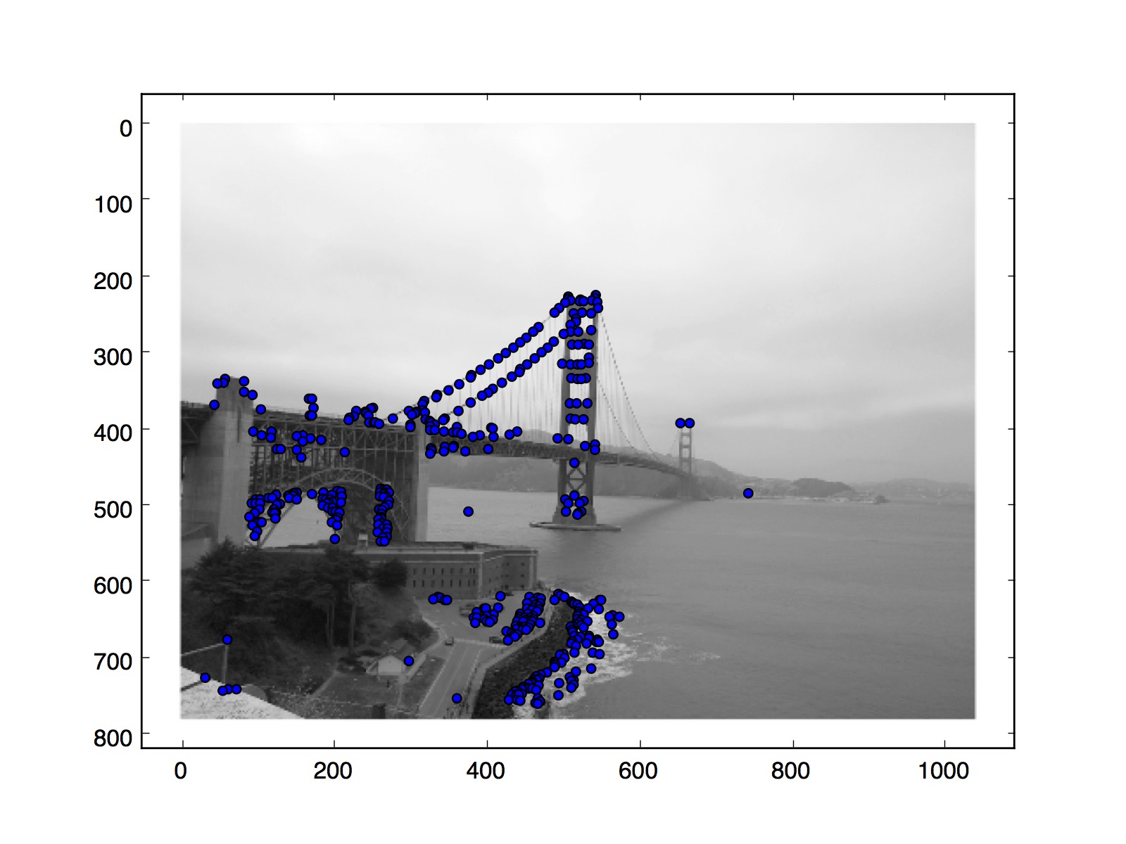
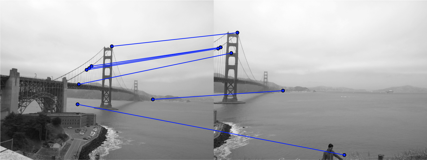
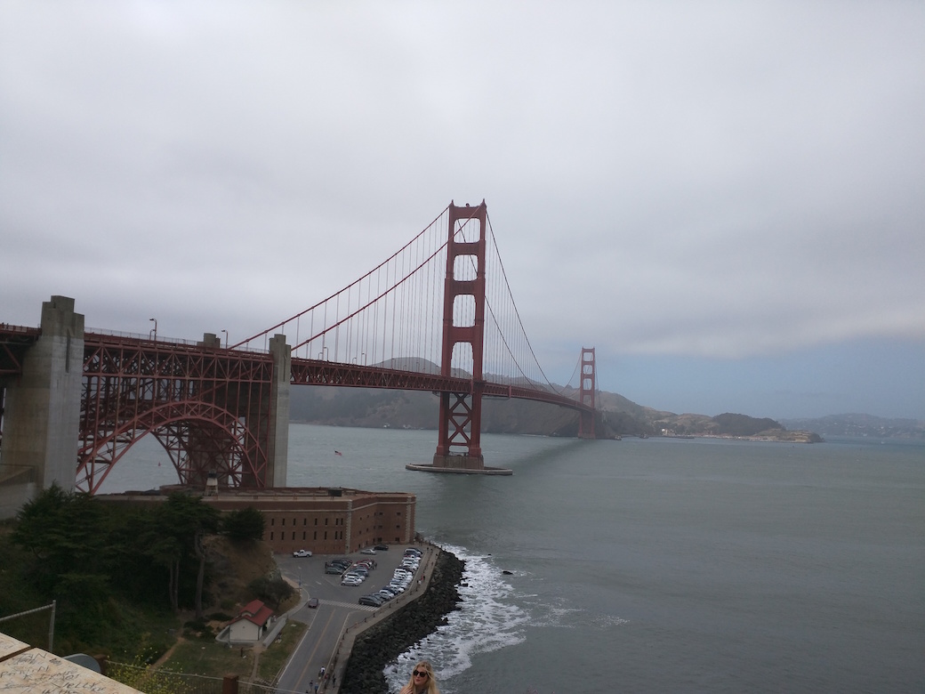Golden Gate on the left

Golden Gate on the right

Golden Gate without blending

Not too bad! Let's see how the linear blended photo compares to that generated by Google Photos.

Golden Gate Manual

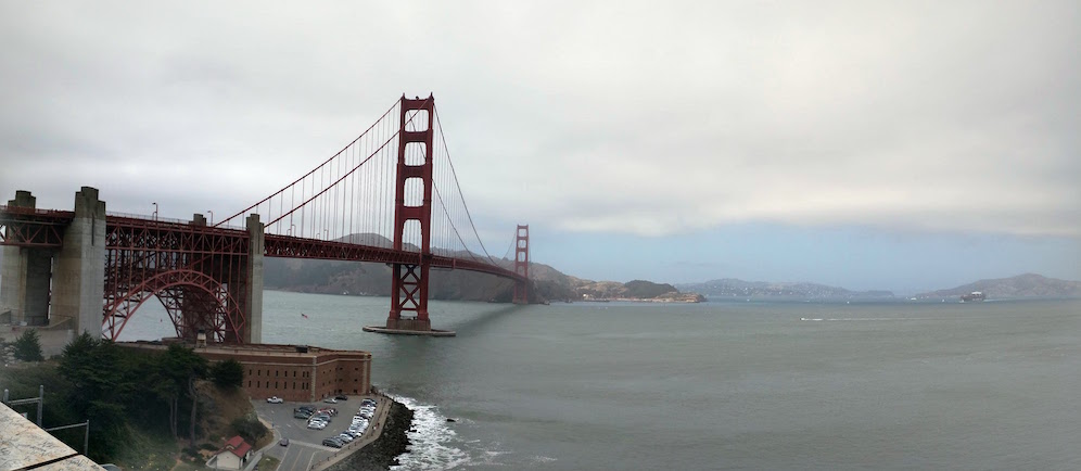Golden Gate Google Photos

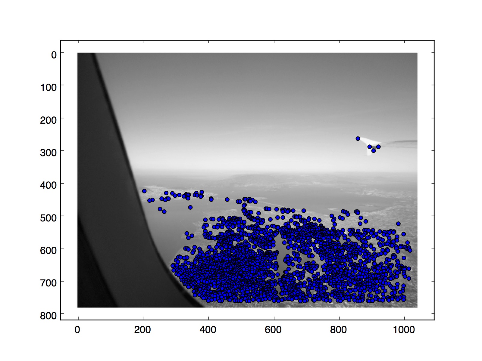
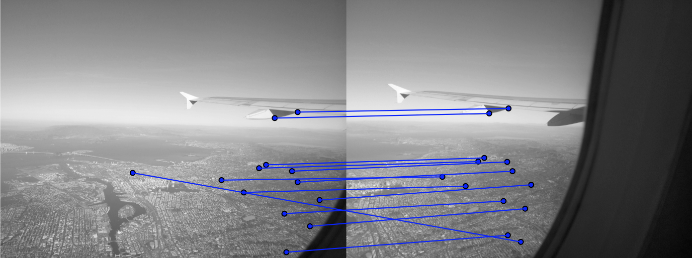
It's really cool how similar they look. Aside from some minor enhancements, we can really see where the panorama came from. Here's another example. As I write this, I'm on a flight to Boston and decided to take a couple of pictures of San Francisco as we were taking off. Aside from the window warping (since the plane's moving quite fast near ground level), this turned out pretty well.

San Francisco Left

San Francisco Center

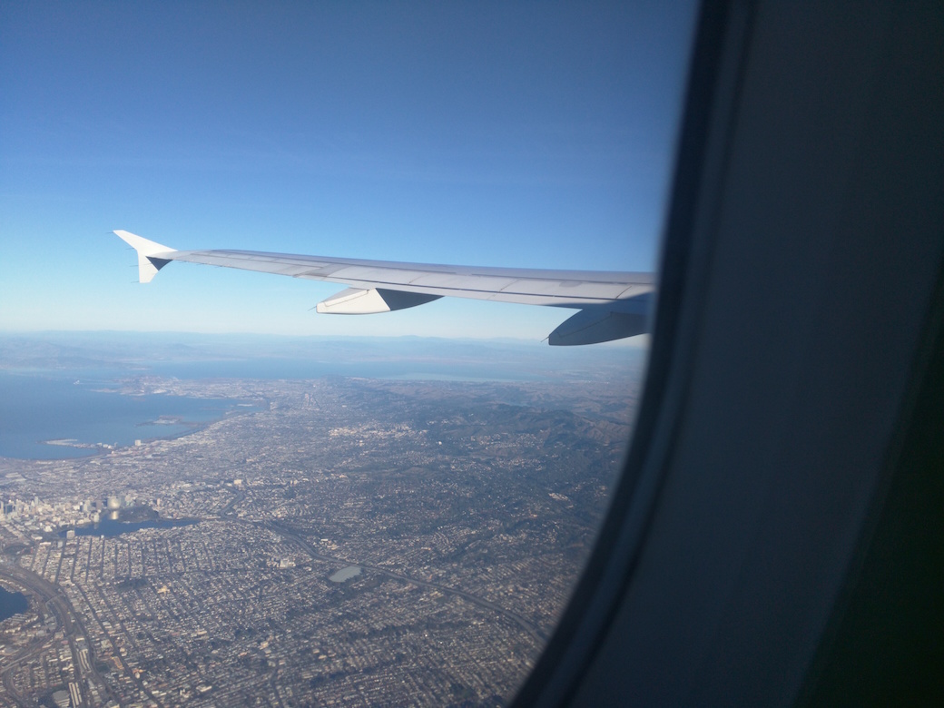San Francisco Right

San Francisco, linear blending

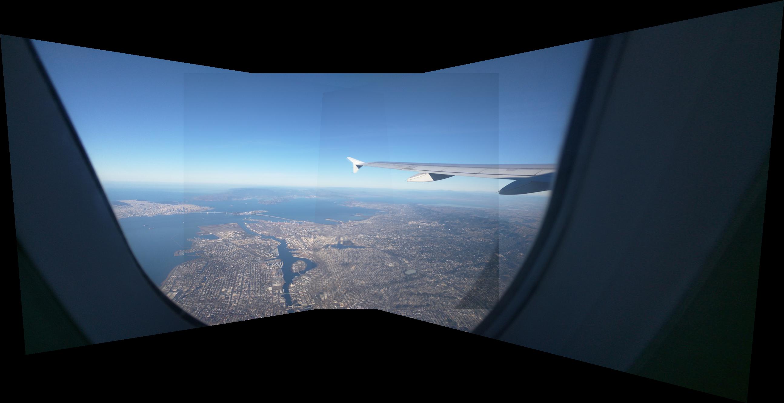San Francsico, Automatic

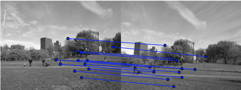
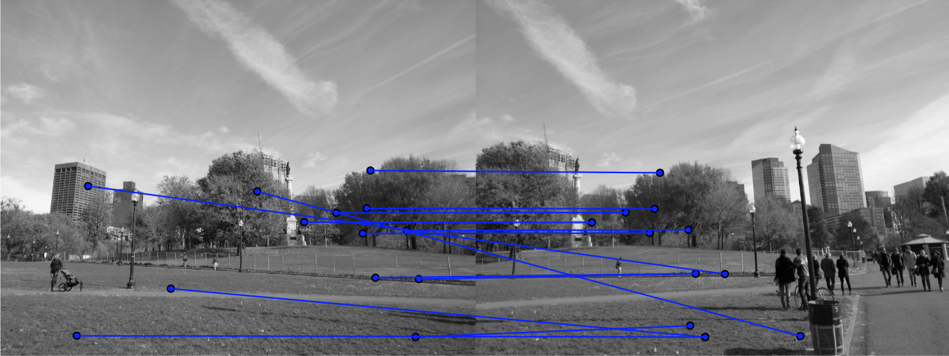
In Boston now! Some more fun pictures!

Boston Common, Left

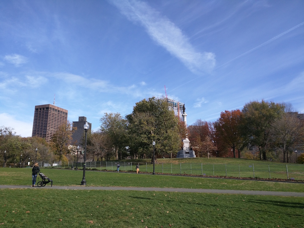Boston Common, Center

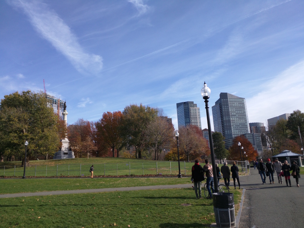Boston Common, Right

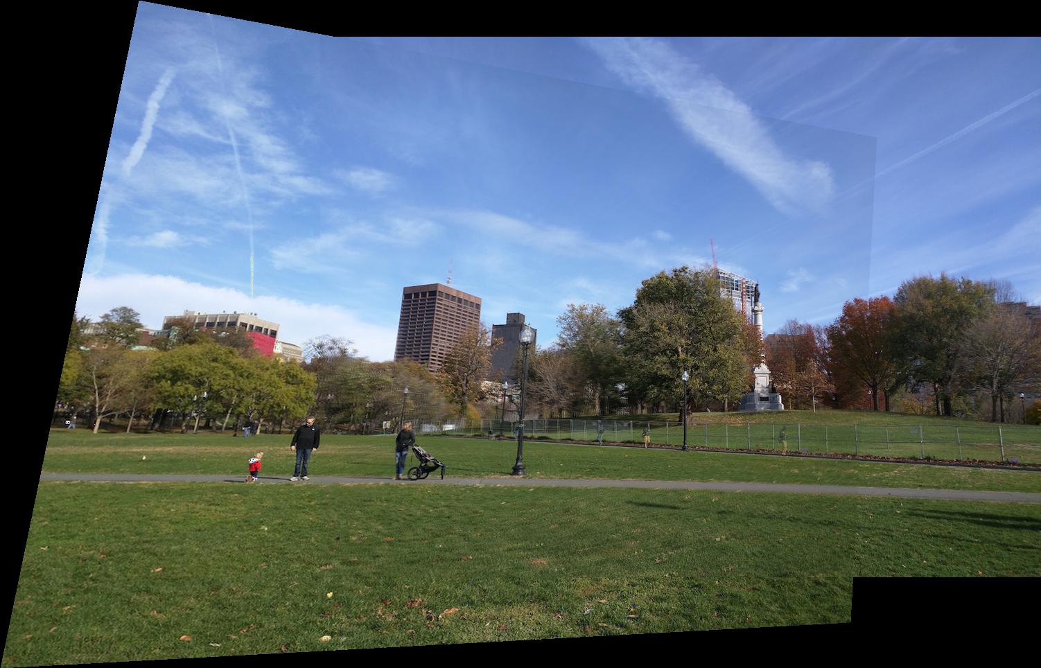
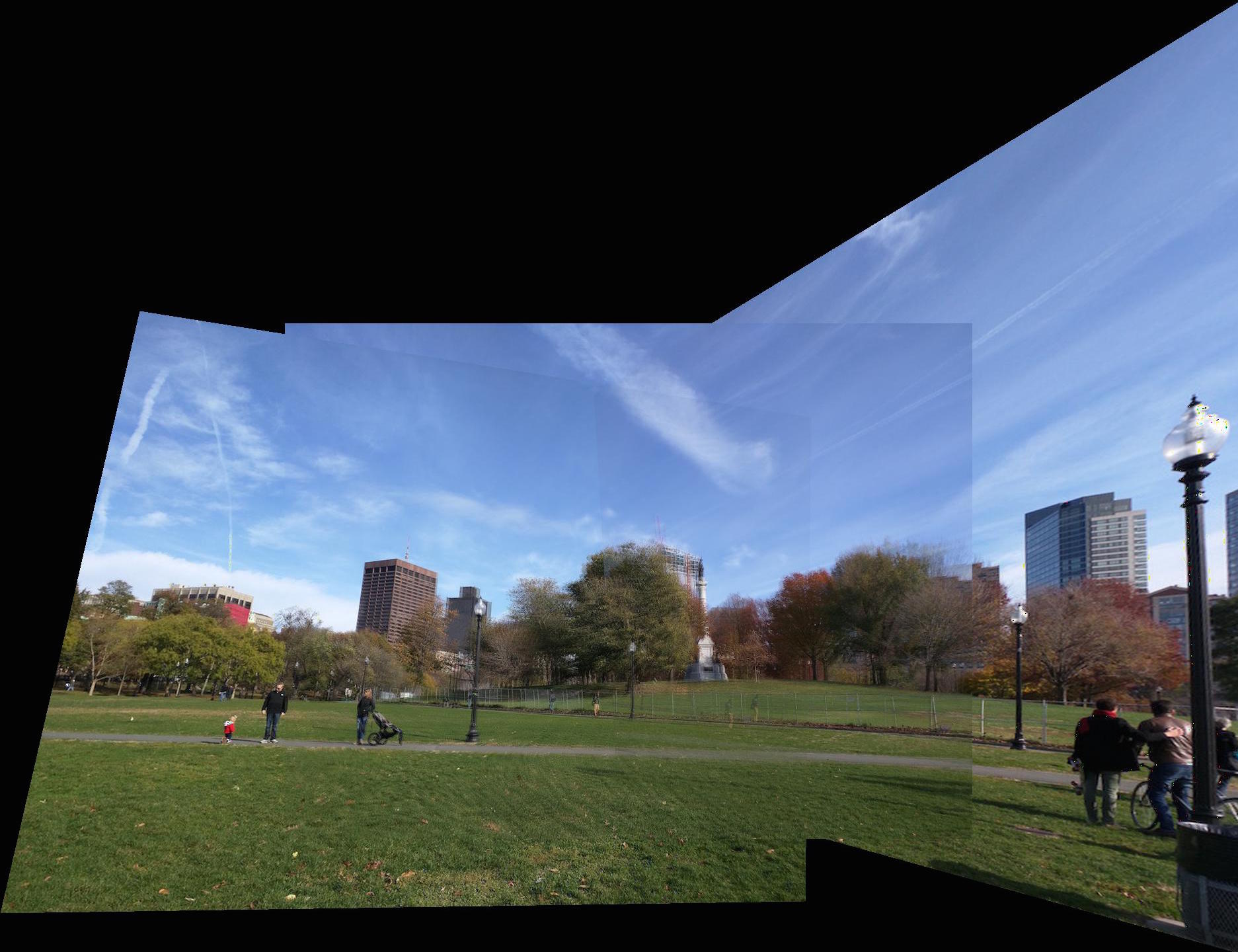Boston Common, Manual

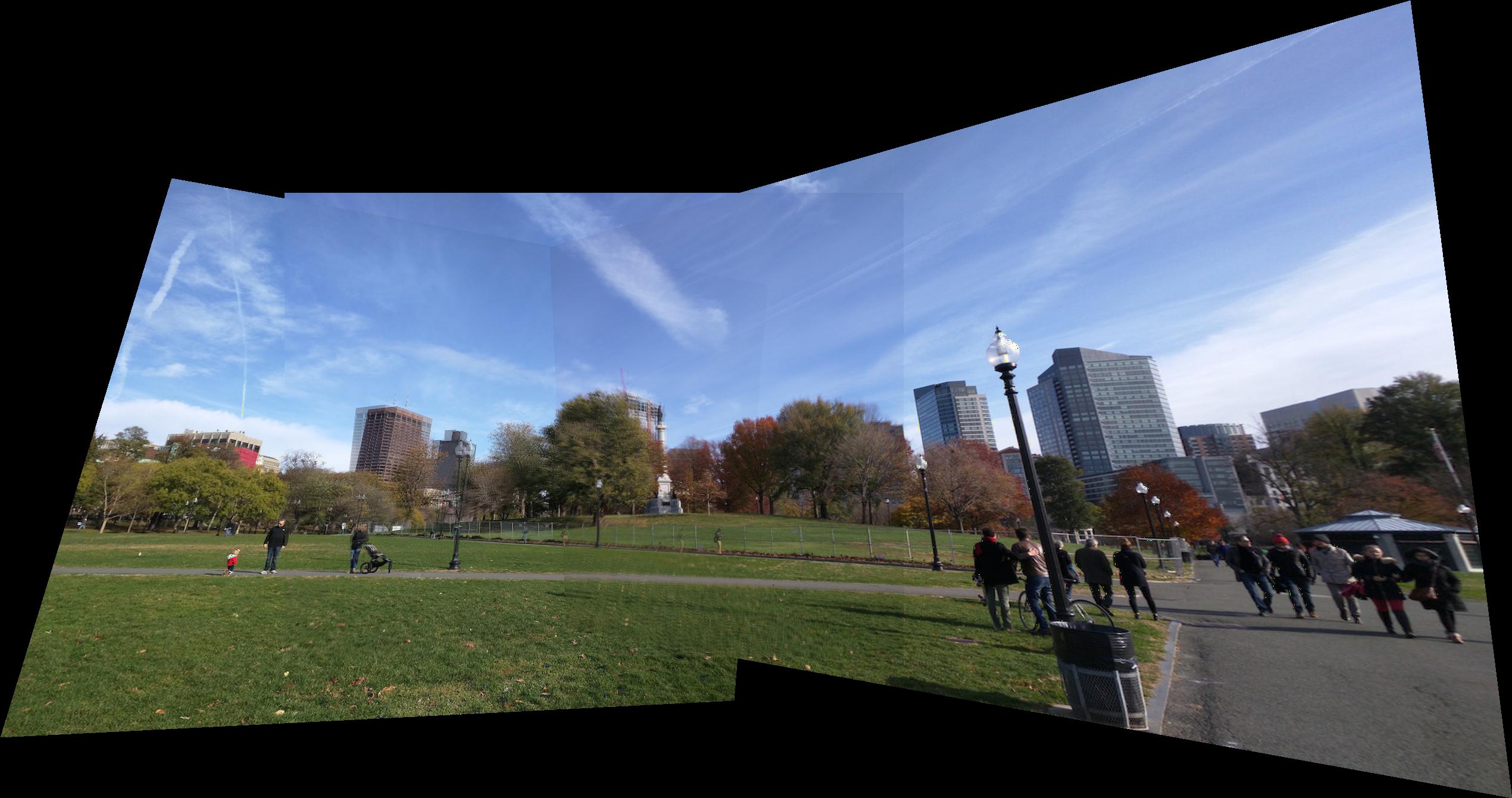Boston Common, Automatic

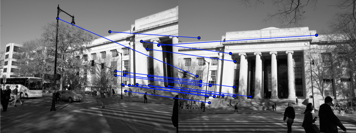
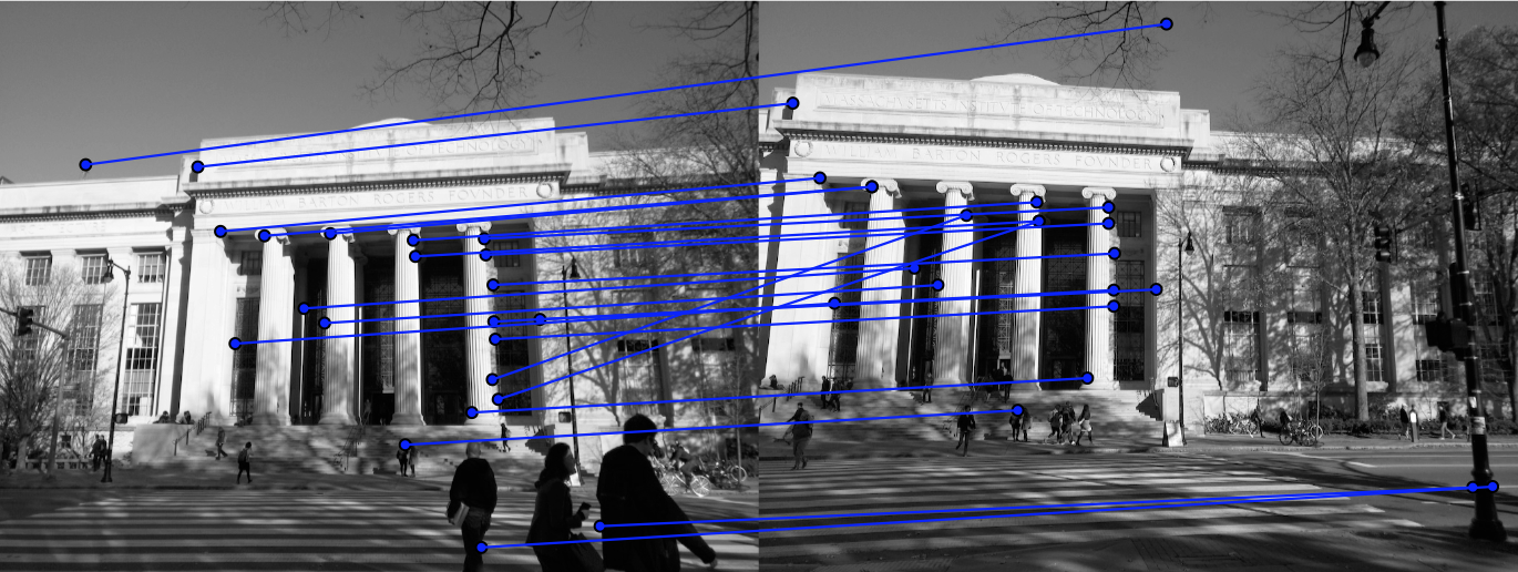
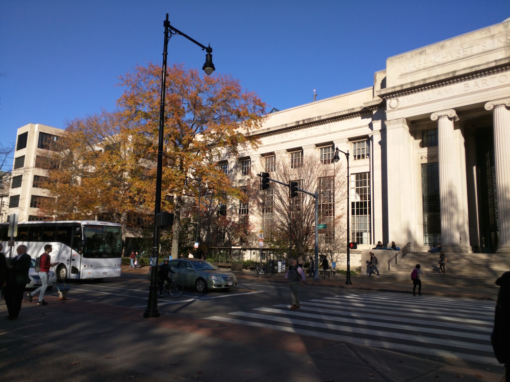MIT, Left

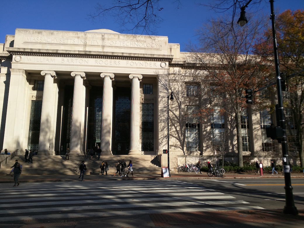
MIT, Center

MIT, Right

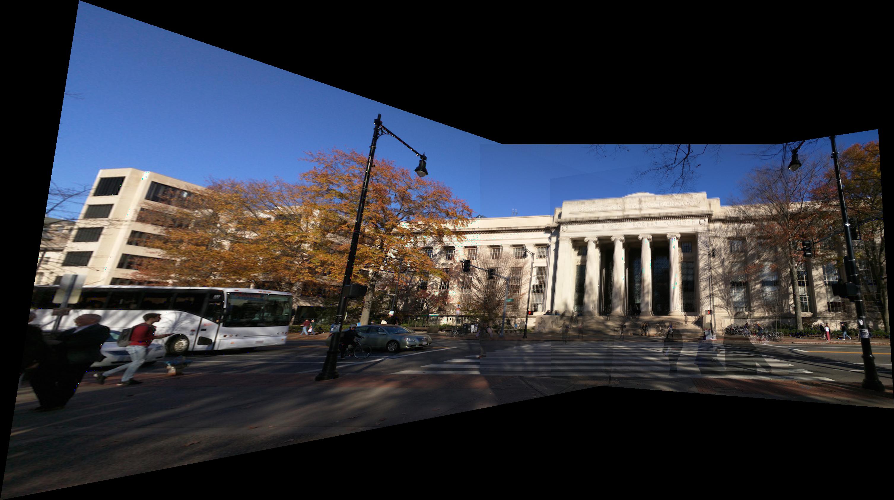MIT, Manual

MIT, Automatic

Bells and Whistles

Texture Insertion

Using basic homographies, I was able to map desired textures onto a scene. Starting with an image of Times Square, I wondered what it would look like if Drake paid for every single billboard for a night.

Times Square

Times Square, Drake-style

Automatic Panorama Generation

To perform automatic panorama generation, I utilized a Bayesian detection scheme. Based on the paper that we discussed in class, I would consider a pair of images part of the same panorama if given n matched points and m inliers, if m > 5.9 + 0.22*n. Given the following images, my code was able to successfully isolate the panoramas from source images (assuming panoramas only made up of a pair of images). It wouldn't be terribly difficult to generalize this code to allow for multiple sources into each panorama.

Plane Center	MIT Center	Boston Left
Plane Right	Golden Gate Left	Boston Center

The results!

Plane, Automatically Discovered

Boston, Automatically Discovered

What I Learned

This project really really made me feel like a kid again. It's so awesome to see how such simple transformations can allow us to create such cool results. Since the release of Google photos, I've always been showing my friends and family some of the cool results it produces. Knowing how to do all of that now makes it that much better.