CS 194-26: Image Manipulation and Computational Photography

Final Project - Gradient Domain Blending and Image Quilting

Giulio Zhou

Gradient Domain Blending

Background

First, let's begin by exploring some of the motivations for gradient domain blending. Recall the blending using Gaussian and Laplacian stacks that we did in project 3. While this was quite useful for blending the seams, an observer would still notice the difference in color if the two images were very different to begin with. As a solution, we operate on the principle that humans are more sensitive to gradients than absolute color intensities. Introducing Poisson blending! Given a source and target image, we will optimize a couple of key criteria.
  1. Source gradients: To ensure that the result maintains the appearance of the source image, we include in our least squares optimization the term ((s_i - s_j) - (x_i - x_j)).
  2. Target border gradients: To seamlessly blend the edges of the source image into the target image, we also include a cross-border term of the form ((x_i - t_j) - (s_i - t_j)).

Part One: Toy Problem

To start, I tested the correctness of the method by inputting its dx/dy gradients into a matrix and optimizing using least squares. If the method was implemented correctly, the result should be exactly the same as the source image. By including the pixel values of the top-left corner, the rest of the intensities fall into place. As we can see, the following two images look more or less the same (minus a small error tolerance).

Toy Problem

Toy Problem Output

Part Two: Poisson Blending

Now that we've verified the correctness of the method, we can move on to the fun stuff! Here, we add in the vertical and leftwards gradients as well (implemented fast in numpy using 
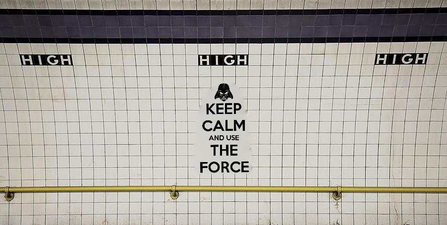
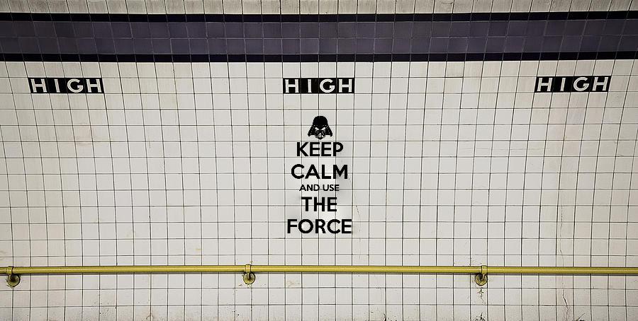
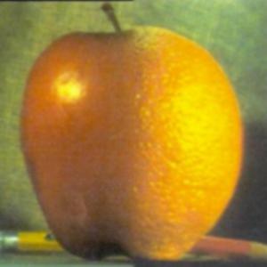
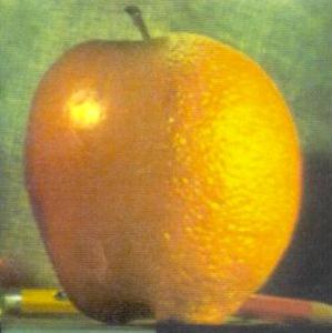
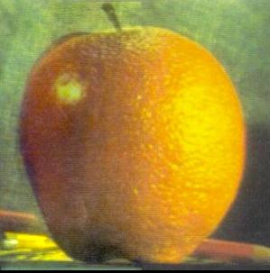
np.roll) into our source matrix and copy in the target gradients into our destination vector b. 
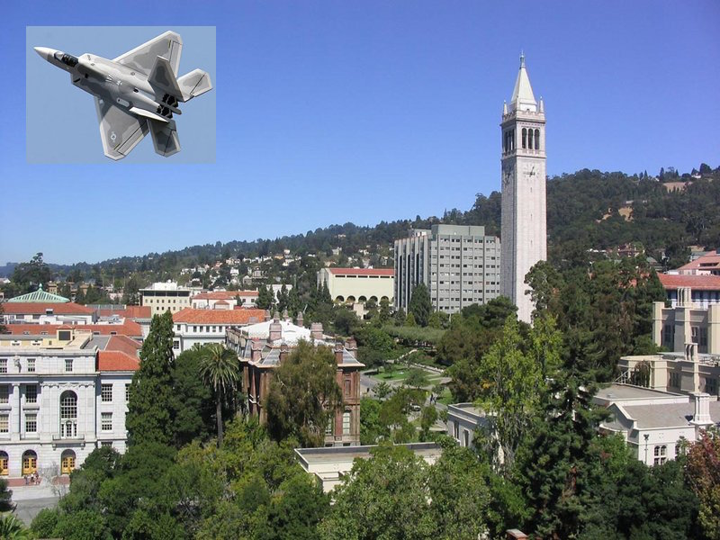
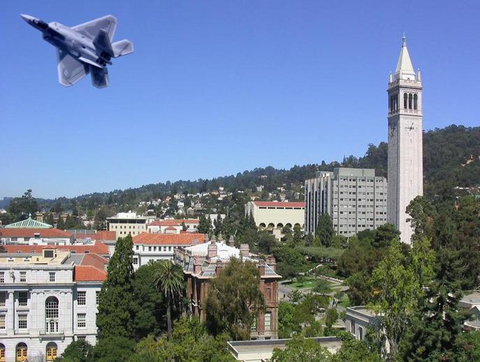
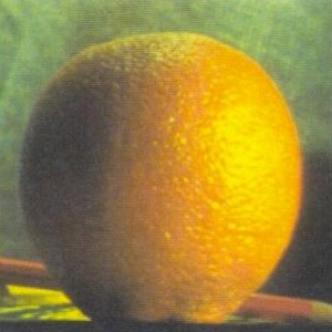
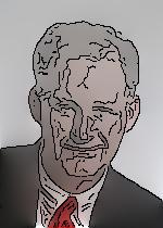
Optimizing with respect to the pixel values for each color channel individually, we obtain some pretty great results!

A Fighter Jet!

Berkeley

Copy-Paste Attempt

It's a plane over Berkeley!

Donald Trump

Shrek

Trump-Shrek

Part Three: Mixed Poisson Blending

As we can see, our results are quite good. So why do we care about this mixed Poisson technique? Consider the case where we want to blend this Keep Calm poster onto the subway surface shown below. Preferably, we'd like to be able to see the background as well. To do so, we try something a little different from Part Two. Instead of optimizing the least squares gradients with respect to just the source image, we instead set it to be equal to the maximum of the target and source gradients by the equation ((x_i - t_j) - max{(s_i - s_j), (t_i - t_j)}).

Keep Calm

Subway

Poisson blending

Mixed Gradient blending
The differences are pretty clear and really cool to see!

Failure Case


Penguin

Suburban House

Penguin House Poisson Blending

Penguin House Mixed Gradient
Notice how the color of the original background makes the penguin extremely dark! Zooming in, we can see that mixed gradients does a slightly better job at preserving the grass gradients but still leads to a rather dark penguin. While gradient domain blending produces fairly good results most of the time, it's clear that blending across wildly differing colors is not it's strong point.

Comparison to Frequency Domain Blending

I tried out our new tools on the apple orange example from the frequency domain blending assignment and found some interesting results.

Apple

Orange

Laplace Blending

Poisson Blending

Mixed Gradient Blending
While mixed gradient blending produced a noticeable ghosting effect, the results from Poisson blending were not half bad! However, we can see how the orange turned the apple somewhat more orange and there is a small seam still visible at the bottom. Based on these observations, it seems that Laplace blending tends to do much better when the colors of the source and target images match and when we want to preserve the absolute intensities of the images. On the other hand, gradient domain blending allows us to perform a much wider array of seamless blends.

Bells and Whistles

Black-and-White Color Remapping

Take a look at the above color-blindness test image. The color version looks cool and all, but the grayscale version has a very prominent issue. We can't actually see the 35! Using the gradient optimization techniques from earlier, we can perform a remapping of the grayscale intensities that increases the contrast of the image while preserving the overall intensities. Mixed gradients help us out a lot here. First, let's examine the image in HSV space. From the results below, it looks like the saturation and value channels are pretty good by themselves. However, it's clearly insufficient to just take the saturation or value channels every time.

Colorblind 35 Test

Colorblind 35 Gray

Colorblind 35 Remapped

Colorblind 73 Test

Colorblind 73 Gray

Colorblind 73 Remapped
As such, we'll try something a little different. Instead of just taking the channel as is, we will approach this as a mixed gradients problem of blending the saturation channel into the value channel.

Texture Smoothing

Playing with gradients gives us a lot of interesting options, allowing us to manipulate high level image features by working with optimizing over relatively lower level features. In this application, I manipulated the image gradients to produce a smoothed out version of the input image. Given this image of Paul Hilfinger, I ran a canny edge detector and only kept gradients at pixels where an edge was detected. The results are quite interesting to behold: it looks like a watercolor painting! Overlaying the detected edges onto the image allows us to really see where the gradients were applied. Although there was some bleeding of colors, it's clear that these were due to the edge detector output, which can easily be manipulated to get the desired output.

Paul Hilfinger

Watercolor Hilfinger

Hilfinger with edges

Barack Obama

Watercolor Obama

Obama with edges

Image Quilting

Texture Synthesis

Random Texture Synthesis

First, I played around with random quilting, where I would generate textures by randomly sampling from the set of available blocks. As we can see below, the results leave very much to be desired. Although it looks quite terrible, this will serve as a benchmark for comparison in the methods we will explore.

Wood Mesh Texture

Random Texture Synthesis

SSD-based Overlap Texture Synthesis

As an improvement to the first method, I implemented a method which overlaps blocks according to a sum of squared distances metric. The difference is noticeable, but the quality is still poor. The seams between the blocks are clearly visible and the sharp color discontinuities are rather terrible.

Wood Mesh Texture

SSD-based Texture Synthesis

Min-Cut Texture Synthesis

Finally, I implemented min-cut texture synthesis to address the issues faced in the previous naive methods of texture synthesis. The method used here is the one discussed in the Image Quilting paper (courtesy of Professor Efros). The algorithm proceeds by generating the texture in raster scan order, using block overlaps of 1/6 the block size. Keeping only the blocks that satisfy some pre-specified overlap constraint s, we compute the minimum cost seam with some randomly chosen block and paste this is into the texture. As we see below, this makes a tremendous difference in the quality of our output textures.


Bells and Whistles

Texture Transfer and Iterative Refinement

Now, some more fun with texture synthesis! Another one of the applications described in Professor Efros' paper, texture transfer involves using pre-specificed textures to paint images by introducing an extra cost term. Previously in the texture synthesis, we worked on minimizing the block overlap error. Here, we define correspondence error, a new term consisting of the squared difference between the Gaussian blurred intensities of the proposed texture block and the corresponding block in the target image.
    
      error = alpha * overlap_error + (1-alpha) * correspondence_error;
    
    
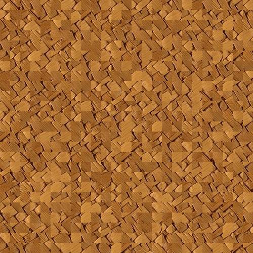
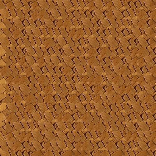
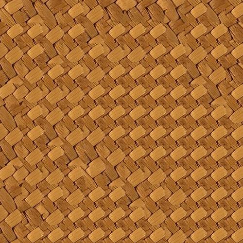
Here are some of the results!

Picasso

Richard Feynman

Feynman as a Picasso painting

Toast

Professor Hilfinger

Startup idea: HilfToaster ™
The results are pretty decent, and were obtained by iterating upon the textures we've already synthesized. Defining a new term, existing_error, as the squared difference between the proposed texture block and the previously synthesized texture, we iterate with a block size reduced by one-third each time and a value of alpha given by
    
      alpha = 0.8 * (i - 1)/(num_iter - 1) + 0.1
    
    
The new error function is given by
    
      error = alpha * (overlap_error + existing_error) + (1-alpha) * correspondence_error;
    
    
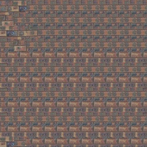
The progression of texture mapping results is shown below.
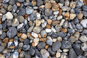
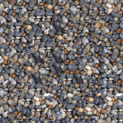
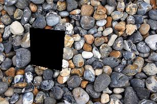
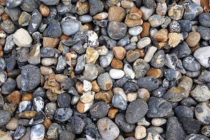
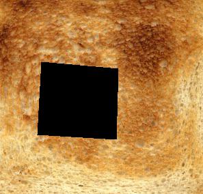
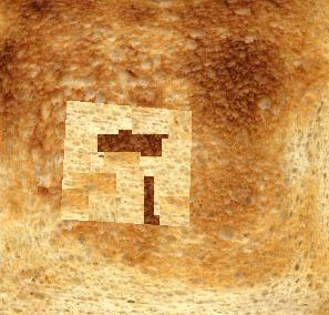


Texture Synthesis for Image Hole Filling

As an experiment, I implemented a naive hole filling algorithm using some of the texture synthesis techniques from earlier. The method takes in an image and the mask to isolate the pixels to be removed. As a rudimentary priority function, I convolve the entire image with a block_size, 
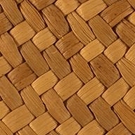
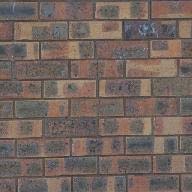
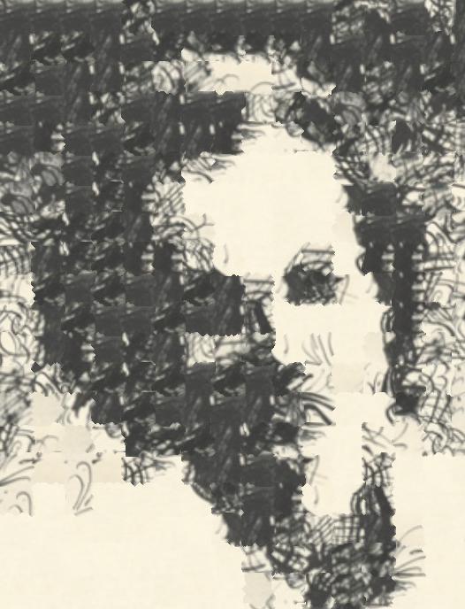
block_size sized array of ones to determine the number of neighbors that each point has, then randomly select one above a certain threshold. Once I've selected the point, I treat this point as the center then get the neighboring pixels. This is matched using an SSD distance metric against other blocks (not sourced from the masked region) and the minimum distance block is used. As we can see, the results are passable but with smarter priority functions and seam blending, the possibilities are certainly endless!

Rocks Fill Iteration 1, Number of Neighbors

Rocks Fill Iteration 2, Number of Neighbors

Rocks Fill Iteration 3, Number of Neighbors


What I Learned

For the first part of the project, I really got a chance to see an application of sparse matrices. Most rows of potentially tens of thousands of entries had just one or two entries, which helped tremendously in terms of computation and memory usage. It's also amazing how subtle manipulation of low level gradient features allow us to generate very interesting high-level changes! In image quilting, it was surprising how such a simple algorithm enabled us to generate such great results. I also really enjoyed getting to replicate some familiar faces with some rather novel textures.